Tutorial

Decorators

@timeit_arg_info_dec

New in v0.1.0

timeit_arg_info_dec is a decorator that decorates a function when it runs, by printing its used parameters, their arguments, the execution time and the output of that function. This can help e.g. with debugging.

[2]:

from typing import List
from time import sleep

import pandas as pd

from extra_ds_tools.decorators.func_decorators import timeit_arg_info_dec

@timeit_arg_info_dec(round_seconds=1)
def illustrate_decorater(a_number: int,
                         text: str,
                         lst: List[int],
                         df: pd.DataFrame,
                         either: bool = True,
                         *args,
                         **kwargs):
    sleep(1)
    return "Look how informative!"

illustrate_decorater(42, 'Bob', list(range(100)), pd.DataFrame([list(range(1,10))]), either=False, **{'Even': 'this works!'})


illustrate_decorater()
---------------------------------------------------------------------------------------------------------------------------------
    param          type_hint                    default_value    arg_type                     arg_value                 arg_len
--  -------------  ---------------------------  ---------------  ---------------------------  ------------------------  ---------
 0  a_number       int                                           int                          42
 1  text           str                                           str                          Bob                       3
 2  lst            List[int]                                     list                         [0, 1, 2,  .. 7, 98, 99]  100
 3  df             pandas.core.frame.DataFrame                   pandas.core.frame.DataFrame                            (1, 9)
 4  either         bool                         True             bool                         False
 5  kwarg['Even']                                                str                          this works!               11

illustrate_decorater()took 1.0 seconds to run.

Returned:
Look how informative!
---------------------------------------------------------------------------------------------------------------------------------

[2]:

'Look how informative!'

For the full documentation of timeit_arg_info_dec click here.

Plots

try_diff_distribution_plots

New in v0.2.0

try_diff_distribution_plots is a function which performs different transformations to a list of numerical values and plots the histogram, probability and the boxplot for each transformation.

[1]:

from numpy.random import default_rng
from extra_ds_tools.plots.eda import try_diff_distribution_plots

rng = default_rng(42)
values = rng.pareto(a=100, size=1000)

fig, axes, transformed_values = try_diff_distribution_plots(values, hist_bins=40)

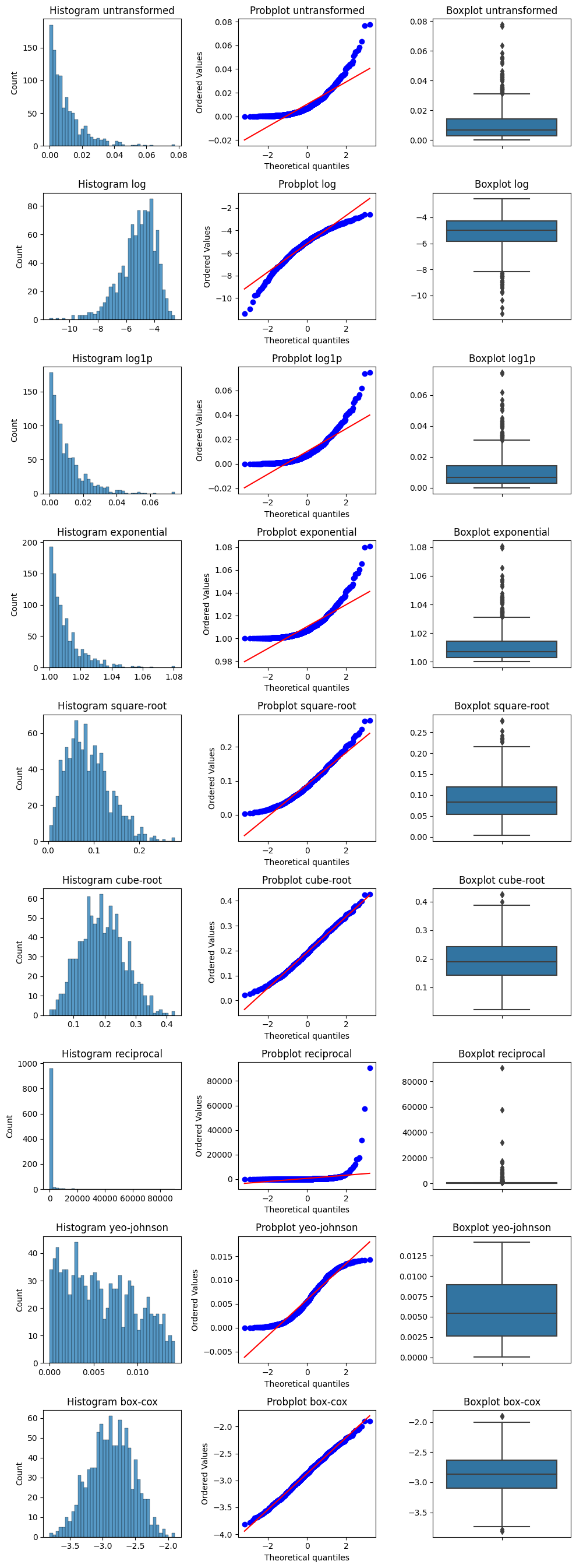
For the full documentation of try_diff_distribution_plots click here.

stripboxplot

New in v0.3.0

stripboxplot is a plot which combines seaborn’s boxplot and stripplot into one plot and adds extra count information using extra-datascience-tool’s add_counts_to_yticks and add_counts_to_xticks.

[4]:

# import libraries
import pandas as pd
import numpy as np

from extra_ds_tools.plots.eda import stripboxplot
from numpy.random import default_rng

# generate data
rng = default_rng(42)
cats = ['Cheetah', 'Leopard', 'Puma']
cats = rng.choice(cats, size=1000)
cats = np.append(cats, [None]*102)
weights = rng.integers(25, 100, size=1000)
weights = np.append(weights, [np.nan]*100)
weights = np.append(weights, np.array([125,135]))
rng.shuffle(cats)
rng.shuffle(weights)
df = pd.DataFrame({'cats': cats, 'weights': weights})
df.head()

[4]:

	cats	weights
0	Cheetah	86.0
1	Puma	38.0
2	Puma	68.0
3	None	NaN
4	Puma	36.0

[5]:

# run stripboxplot
fig, ax = stripboxplot(df, 'cats', 'weights')

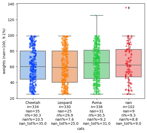
For the full documentation of stripboxplot click here.

add_counts_to_xticks

New in v0.3.0

add_counts_to_xticks is a function which add count statistics of a categorical variable on the x-axis of a plot. If the categorical variable is on the y-axis you can use add_counts_to_yticks instead.

[1]:

# import libraries
import matplotlib.pyplot as plt
import seaborn as sns
import pandas as pd
import numpy as np

from extra_ds_tools.plots.format import add_counts_to_xticks
from numpy.random import default_rng

# generate data
rng = default_rng(42)
cats = ['Cheetah', 'Leopard', 'Puma']
cats = rng.choice(cats, size=1000)
cats = np.append(cats, [None]*102)
weights = rng.integers(25, 100, size=1000)
weights = np.append(weights, [np.nan]*100)
weights = np.append(weights, np.array([125,135]))
rng.shuffle(cats)
rng.shuffle(weights)
df = pd.DataFrame({'cats': cats, 'weights': weights})
df.head()

[1]:

	cats	weights
0	Cheetah	86.0
1	Puma	38.0
2	Puma	68.0
3	None	NaN
4	Puma	36.0

Create e.g. a violinplot

[2]:

fig, ax = plt.subplots()
sns.violinplot(df, x='cats', y='weights', ax=ax)

[2]:

<AxesSubplot: xlabel='cats', ylabel='weights'>

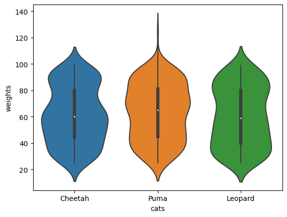
Add counts to the x-ticks

[3]:

fig, ax = add_counts_to_xticks(fig, ax, df, x_col='cats', y_col='weights')
fig

[3]:

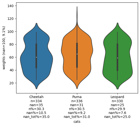
For the full documentation of add_counts_to_xticks click here.

ML

filter_tried_params

New in v0.4.0

filter_tried_params is a function which filters out previously tried parameters in a GridSearchCV if the model is otherwise identical. This can save a lot of time because you won’t be rerunning already tried settings.

[1]:

# import libraries
from sklearn.model_selection import GridSearchCV
from sklearn.tree import DecisionTreeRegressor
from sklearn.pipeline import make_pipeline

from extra_ds_tools.ml.sklearn.model_selection import filter_tried_params

model = make_pipeline(DecisionTreeRegressor())

new_param_grid = {
    "decisiontreeregressor__max_depth": [1, 2],
    "decisiontreeregressor__splitter": ["best", "random"],
}
new_gridsearch = GridSearchCV(model, new_param_grid)

# initiate two other GridsearchCVs, we assume we have ran them already
tried_param_grid1 = {
    "decisiontreeregressor__max_depth": [2, 3],
    "decisiontreeregressor__splitter": ["best", "random"],
}
tried_param_grid2 = {
    "decisiontreeregressor__max_depth": [3, 4],
    "decisiontreeregressor__splitter": ["best", "random"],
}
tried_gridsearches = [
    GridSearchCV(model, tried_param_grid1),
    GridSearchCV(model, tried_param_grid2)
]

# change the param grid of the new GridSearchCV to the filtered param grid
untried_param_grid = filter_tried_params(gridsearchcv=new_gridsearch, tried_gridsearches=tried_gridsearches)
new_gridsearch.param_grid = untried_param_grid
new_gridsearch.param_grid

[1]:

[{'decisiontreeregressor__max_depth': [1],
  'decisiontreeregressor__splitter': ['best']},
 {'decisiontreeregressor__max_depth': [1],
  'decisiontreeregressor__splitter': ['random']}]

As you can see above, the new GridSearchCV will only run the two new options it hasn’t tried before.

For the full documentation of filter_tried_params click here.

EstimatorSwitch

New in v0.5.0

EstimatorSwitch is a meta-estimator that can turn on or off other estimators/transformers in a scikit-learn Pipeline. This can e.g. be useful when testing for the impact of a feature-engineering estimator/transformer with a GridSearchCV.

[1]:

# import libraries
import numpy as np

from sklearn.pipeline import Pipeline
from feature_engine.imputation import MeanMedianImputer, ArbitraryNumberImputer

from extra_ds_tools.ml.sklearn.meta_estimators import EstimatorSwitch

# create X and y
X = np.array([np.nan, 10] * 5).reshape(-1,1)
y = np.array([5, 10] * 5).reshape(-1, 1)

# create pipeline steps
pipeline = Pipeline(
    [("medianimputer", EstimatorSwitch(MeanMedianImputer(), apply=False)),
    ("arbitraryimputer", EstimatorSwitch(ArbitraryNumberImputer(-1), apply=True))]
)

# transform X according to pipeline
pipeline.fit_transform(X)

[1]:

	x0
0	-1.0
1	10.0
2	-1.0
3	10.0
4	-1.0
5	10.0
6	-1.0
7	10.0
8	-1.0
9	10.0

Above you can see that the nan values have not been imputed with the mean: 10, but with the arbitrary number -1 because we used EstimatorSwitch to turn off the MeanMedianImputer.

To use EstimatorSwitch to turn off estimators/transformers during a GridSearchCV:

[2]:

import pandas as pd

from sklearn.tree import DecisionTreeRegressor
from sklearn.model_selection import GridSearchCV
from sklearn.pipeline import Pipeline

from feature_engine.imputation import MeanMedianImputer, ArbitraryNumberImputer

from extra_ds_tools.ml.sklearn.meta_estimators import EstimatorSwitch

[3]:

clf = Pipeline(
    [("meanmedianimputer", EstimatorSwitch(MeanMedianImputer())),
    ("arbitraryimputer", EstimatorSwitch(ArbitraryNumberImputer(-1))),
    ("tree", DecisionTreeRegressor())]
)
clf

[3]:

Pipeline(steps=[('meanmedianimputer',
                 EstimatorSwitch(estimator=MeanMedianImputer())),
                ('arbitraryimputer',
                 EstimatorSwitch(estimator=ArbitraryNumberImputer(arbitrary_number=-1))),
                ('tree', DecisionTreeRegressor())])

In a Jupyter environment, please rerun this cell to show the HTML representation or trust the notebook.
On GitHub, the HTML representation is unable to render, please try loading this page with nbviewer.org.

Use the get_params() method to get the right parameters for the parameter grid for the GridSearchCV.

[4]:

clf.get_params()

[4]:

{'memory': None,
 'steps': [('meanmedianimputer',
   EstimatorSwitch(estimator=MeanMedianImputer())),
  ('arbitraryimputer',
   EstimatorSwitch(estimator=ArbitraryNumberImputer(arbitrary_number=-1))),
  ('tree', DecisionTreeRegressor())],
 'verbose': False,
 'meanmedianimputer': EstimatorSwitch(estimator=MeanMedianImputer()),
 'arbitraryimputer': EstimatorSwitch(estimator=ArbitraryNumberImputer(arbitrary_number=-1)),
 'tree': DecisionTreeRegressor(),
 'meanmedianimputer__apply': True,
 'meanmedianimputer__estimator__imputation_method': 'median',
 'meanmedianimputer__estimator__variables': None,
 'meanmedianimputer__estimator': MeanMedianImputer(),
 'arbitraryimputer__apply': True,
 'arbitraryimputer__estimator__arbitrary_number': -1,
 'arbitraryimputer__estimator__imputer_dict': None,
 'arbitraryimputer__estimator__variables': None,
 'arbitraryimputer__estimator': ArbitraryNumberImputer(arbitrary_number=-1),
 'tree__ccp_alpha': 0.0,
 'tree__criterion': 'squared_error',
 'tree__max_depth': None,
 'tree__max_features': None,
 'tree__max_leaf_nodes': None,
 'tree__min_impurity_decrease': 0.0,
 'tree__min_samples_leaf': 1,
 'tree__min_samples_split': 2,
 'tree__min_weight_fraction_leaf': 0.0,
 'tree__random_state': None,
 'tree__splitter': 'best'}

Create a parameter grid with MeanMedianImputer and the ArbitraryNumberImputer turned off and on seperately using the apply parameter of EstimatorSwitch.

[5]:

param_grid = [
        {
            "meanmedianimputer__apply": [True],
            "meanmedianimputer__estimator__imputation_method": ["mean", "median"],
            "arbitraryimputer__apply": [False]
        },
        {
            "arbitraryimputer__apply": [True],
            "arbitraryimputer__estimator__arbitrary_number": [-1],
            "meanmedianimputer__apply": [False]
        }
]

[6]:

gridsearch = GridSearchCV(estimator=clf, param_grid=param_grid)
gridsearch.fit(X,y)
pd.DataFrame(gridsearch.cv_results_)

[6]:

	mean_fit_time	std_fit_time	mean_score_time	std_score_time	param_arbitraryimputer__apply	param_meanmedianimputer__apply	param_meanmedianimputer__estimator__imputation_method	param_arbitraryimputer__estimator__arbitrary_number	params	split0_test_score	split1_test_score	split2_test_score	split3_test_score	split4_test_score	mean_test_score	rank_test_score
0	0.001864	0.000288	0.001197	0.000127	False	True	mean	NaN	{'arbitraryimputer__apply': False, 'meanmedian...	0.0	0.0	0.0	0.0	0.0	0.0	2
1	0.001910	0.000170	0.001023	0.000098	False	True	median	NaN	{'arbitraryimputer__apply': False, 'meanmedian...	0.0	0.0	0.0	0.0	0.0	0.0	2
2	0.001154	0.000081	0.000985	0.000176	True	False	NaN	-1	{'arbitraryimputer__apply': True, 'arbitraryim...	1.0	1.0	1.0	1.0	1.0	1.0	1

For the full documentation of EstimatorSwitch click here.